Researcher, Department of Mathematics and Computer Science, University of Basel
Java continues to be a challenge on the OSX platform. We have recently experienced just how sensitive Scalismo is to using the correct Java version.
As explained in the setup guide, we encourage people to install the Zulu version 11.0-9 of JVM using the command line.
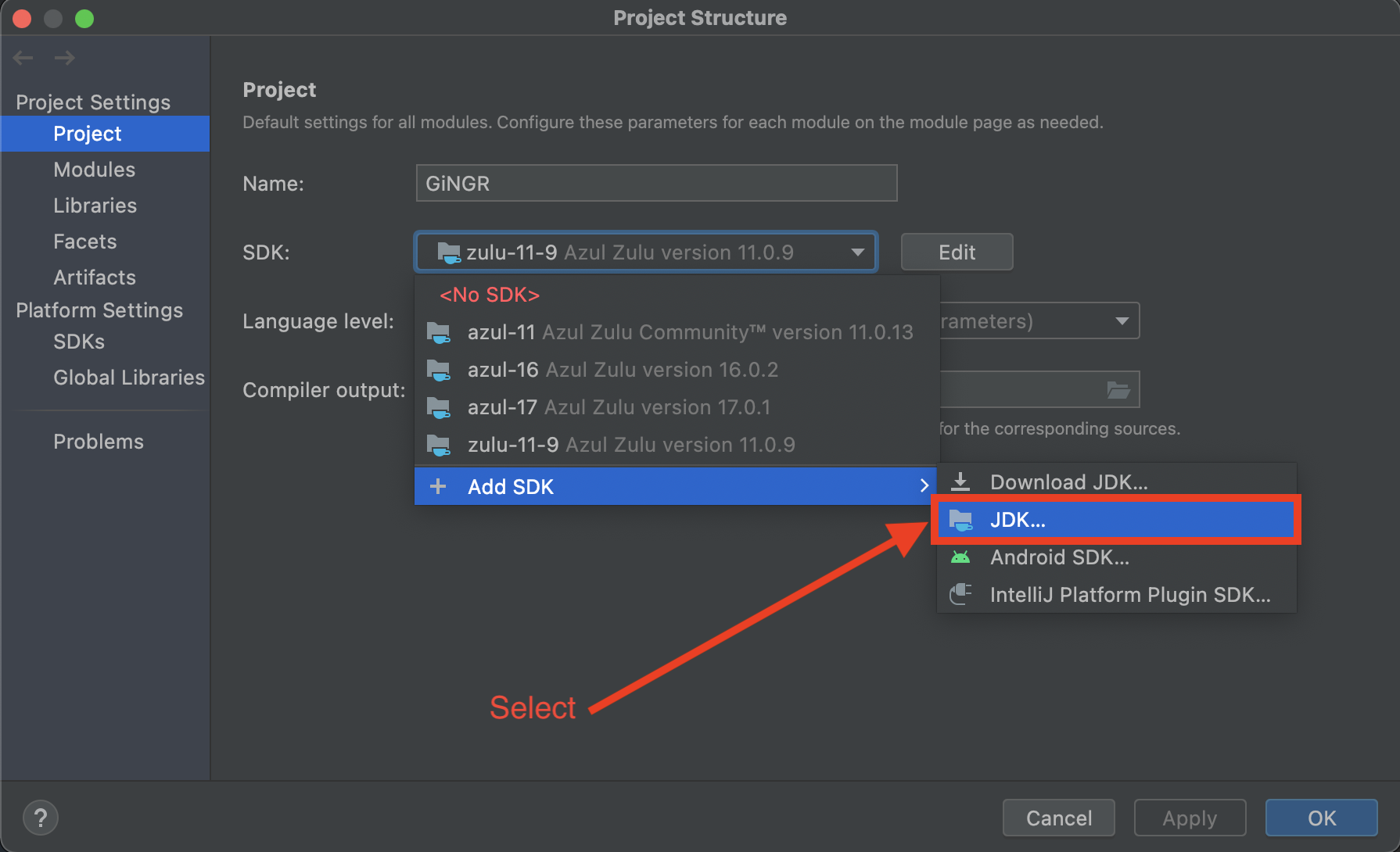
However, when using Zulu JDK in IntelliJ, there is no option to select the specific minor version 9. Unfortunately, the newest version does not always work and might result in the following error when initializing Scalismo:
libc++abi: terminating with uncaught exception of type NSException

Process finished with exit code 134 (interrupted by signal 6: SIGABRT)
To fix this, we have to manually import the Zulu 11.0-9 JDK downloaded with Coursier from the command line. To do so, we need to know the java.home directory. This can be found by starting sbt and invoking:
The recently released version of Scalismo - version 0.90 - comes with a number of important changes in its
core classes. In this blog post, we will look at images.
In older versions of Scalismo images had a special status in the library. While conceptually they were thought to be just discrete fields, they were implemented using a number of special classes, representing the differnet types of images.
This led to inconsistencies in the
API and complicated the type hierarchy. Even worse, it enforced the wrong notion that image are conceptually different from other representations of
intensities used in Scalismo. In version 0.90 we cleaned up the hierarchy and removed all the special classes. Discrete images are now simply a special instantiation of a discrete field, whose
domain is a regular grid. In the following we explain the underlying concepts, show how we can create images and how
we can obtain a continuous from a discrete representations and vice versa.
Similar to other types of representations, images come in two types: Discrete images and continuous images.
Continuous images are modeled as a Field; I.e. they are functions that have a domain $$D \subset \mathbb{R}^d$$ and
map each point of the domain to some values. The mapped values can be scalars, vectors or even more complicated objects.
Discrete images in turn are a special case of a discrete field. Discrete fields are defined as a finite set of points, where for each point we have an associated value.
A discrete image is a discrete field, whose domain is constrained to be a regular grid; I.e. whose domain points are equally spaced. That the points are equally spaces makes
it possible to represent the domain points implicitly by a mathematical formula rather than having to explicitly store them.
Furthermore, accessing the image values and looking up closest points becomes a constant time operation.
The basic object to represent such a set of structured points is the class StructuredPoints.
We can create a set of points on a grid as follows:
val origin = Point3D(10.0, 15.0, 7.0) // some point defining the lower left corner of the image
val spacing = EuclideanVector3D(0.1, 0.1, 0.1) // the spacing between two grid points in each space dimension
val size = IntVector3D(32, 64, 92) // size in each space dimension
val points = StructuredPoints3D(origin, spacing, size)
This creates a grid of points $$32 \times 64 \times 92$$ points, where the bottom left point is at the origin,
and the points are the in the $$x, y, z$$ direction $$0.1mm$$ apart.
Note that the grid of points is aligned to the coordinate axis. In case you would like to have a different
alignment, it is possible to specify a rotation of the points. The rotation is specified by 1 or 3 Euler angles,
depending on whether there is a 2 or 3 dimensional image.
val yaw = Math.PI / 2
val pitch = 0.0
val roll = Math.PI
val points2 = StructuredPoints3D(origin, spacing, size, yaw, pitch, roll)
The image domain represents a domain, whose points are aligned in a rectangular grid.
Naturally, it uses StructuredPoints as a representation of the underlying points of the
domain. We can create an image domain from structured points as follows:
val imageDomain = DiscreteImageDomain3D(StructuredPoints3D(origin, spacing, size))
For convenience, Scalismo also offers the possibility to specify the origin, spacing and size directly, as we did
for the structured points.
val imageDomain2 = DiscreteImageDomain3D(origin, spacing, size)
Note however, that this still creates a structured points object internally.
As for structured points, we can also define a rotation, by specifying the corresponding
Euler angles.
val imageDomain3 = DiscreteImageDomain3D(origin, spacing, size, yaw, pitch, roll)
Finally, we can specify the points by specifying its bounding box together with the information about the spacing or size:
val boundingBox : BoxDomain[_3D] = imageDomain.boundingBox
val imageDomain4 = DiscreteImageDomain3D(boundingBox, spacing = spacing)
or
val imageDomain5 = DiscreteImageDomain3D(boundingBox, size = size)
This last creation method is particularly useful for changing the resolution of an image,
as we will see later.
To create an image, we need to specify a value for each
point in the domain. In this example, we create an image, which assigns a zero value to each point.
val image = DiscreteImage3D(imageDomain, p => 0.toShort)
Alternatively, we could have specified the values using an array, as follows:
val image2 = DiscreteImage3D(imageDomain, Array.fill(imageDomain.pointSet.numberOfPoints)(0.toShort))
Note that an image is just another name for a discrete field with a image domain. We could
have equally well constructed the image as:
val image3 = DiscreteField3D(imageDomain, p => 0.toShort)
It is often more convenient to work with a continuous representation of the image.
To obtain a continuous image, we use the interpolate method and specify a suitable
interpolator:
val continuousImage : Field[_3D, Short] = image.interpolate(BSplineImageInterpolator3D(degree = 3))
The resulting object is defined on all the points within the bounding box of the image domain.
To go back to a discrete representation, we can specify a new image domain and use the
discretize method. As the new domain could be bigger than the domain of the continuous image,
we need to specify a value that is assigned to the points, which fall outside this domain.
val newDomain = DiscreteImageDomain3D(image.domain.boundingBox, size=IntVector(32, 32, 32))
val resampledImage : DiscreteImage[_3D, Short] = continuousImage.discretize(newDomain, outsideValue = 0.toShort)
Of course, we could also resample the continuous image using a different type of domain. Assume for example that we
have a CT image of the upper leg, but we are only interested in representing the intensities for the femur bone. We could then
discretize the (interpolated) image using a tetrahederal mesh, and thus obtain a representation of the field which is restricted
to the femur bone only.
val femurMesh : TetrahedralMesh[_3D] = ???
val femurVolumeMeshModel : DiscreteField[_3D, TetrahedralMesh, Short] = continuousImage.discretize(femurMesh)
We have discussed the new design of images in Scalismo. Discrete images are modelled as discrete fields, and thus have a domain and
associated values attached to it. The points of the domain are represented using the class StructuredPoints, which
represent points that lie on a regular grid. Exploiting this special structure, we can efficiently access values
associated to the grid points in the image, or use dedicated interpolation methods to swich from a discrete to a
continuous representation. Once we have the continuous representation, we can discretize using a different domain, which
allows us for example to resample the image in a different resolution, restrict the image to a part of the domain or even change the
type of the domain.
The recently released version of Scalismo - version 0.90 - comes with a number of important changes in its
core classes. In this blog post we will look at the class PointDistributionModel, which replaces and
generalizes StatisticalMeshModel.
We start by discussing the differences to the previous implementation. We then show how to create Point Distribution Models.
In the last part we will discuss how we can change the domain over which the Point Distribution Model is defined. This allows us to change
the resolution of the model, restrict the model to a subset of the original domain, or even to change the type of domain over which the model is defined.
From StatisticalMeshModel to PointDistributionModel
Recall that shape variations are modelled using Gaussian processes in Scalismo. More precisely,
we use a low-rank approximation of a Gaussian process, which models a probability distribution over deformation fields,
val lowrankGP : LowRankGaussianProcess[_3D, EuclideanVector[_3D]] = ???
The type signature indicates that the Gaussian process is defined in 3D space and it represents a
collection of random variables over 3D vectors in Euclidean space.
A StatisticalMeshModel is the restriction of this continuously defined Gaussian Process to
a discrete and finite set of points. This set of points is defined to be the vertices of a triangle mesh,
which is called the reference mesh.
Thus, a StatisticalMeshModel is just an aggregate of a mesh and a corresponding Gaussian process,
restricted to the points of the reference mesh. This is reflected in the definition in Scalismo:
case class StatisticalMeshModel (referenceMesh: TriangleMesh[_3D],
                                 gp: DiscreteLowRankGaussianProcess[_3D, TriangleMesh, EuclideanVector[_3D]])
When we draw a sample from this model, we actually draw a sample from the Gaussian process and apply
the sampled deformation field to the points of the reference mesh. The resulting sample is the deformed version of the reference mesh.
val ssm : StatisticalMeshModel = ???
val sample : TriangleMesh[_3D] = ssm.sample
From this description it becomes obvious how we can generalize this to other types of datasets.
As we only use the points of the mesh, we can relax the restriction that the reference has to be a triangle mesh.
Instead, we assume that the dataset is defined on a finite set of points. In Scalismo, a dataset which is defined on
a finite set of points is modelled as a subtype of the class DiscreteDomain. This is the basis of the definition of
a PointDistributionModel:
case class PointDistributionModel[D, DDomain[D] <: DiscreteDomain[D]](
    reference : DDomain[D],
    gp: DiscreteLowRankGaussianProcess[D, DDomain, EuclideanVector[D]]
 ) (implicit warper: DomainWarp[D, DDomain])
Here we replaced TriangleMesh by the generic type DDomain, which can be any subtype
of a DiscreteDomain. The implicit argument warper restricts the domains further to domains
that can be deformed. In Scalismo these are currently the classes TriangleMesh,
TetrahedralMesh, LineMesh and UnstructuredPointsDomain.1
In the actual Scalismo implementation, the definition of the class PointDistributionModel is even a bit simpler.
The reference is assumed to coincide with the domain over which the (discrete) Gaussian process is defined. Therefore,
we do not even need to explicitly represent it as part of the class PointDistributionModel.
Creating and working with Point Distribution Models
Now that we know what a Point Distribution Model is, we will show how we work with them in Scalismo.
Our first example illustrates how to learn a Point Distribution Model of tetrahedral meshes from given example meshes.
This is simple: We create a data collection, where we provide a sequence of tetrahedral meshes and use the method createUsingPCA
to create the model:
val referenceMesh: TetrahedralMesh[_3D] = ???
val trainingMeshes: Seq[TetrahedralMesh[_3D]] = ???
val dataCollection = DataCollection.fromTetrahedralMeshSequence(referenceMesh, trainingMeshes)
val pdmTetraMesh = PointDistributionModel.createUsingPCA(dataCollection)
As expected, samples from this model are valid tetrahedral meshes.
val sample: scalismo.mesh.TetrahedralMesh[_3D] = pdmTetraMesh.sample()
Creating models of other types of data sets works exactly in the same way. We simply change the corresponding type
of the reference and the data collection.
val referenceMesh: TriangleMesh[_3D] = ???
val trainingMeshes: Seq[TriangleMesh[_3D]] = ???
val dataCollection = DataCollection.fromTriangleMeshSequence(referenceMesh, trainingMeshes)
val pdmTriangleMesh = PointDistributionModel.createUsingPCA(dataCollection)
A second way to create a PDMs is to specify a low rank Gaussian process as well as a reference mesh on which
the Gp will be discretized:
val lowRankGP : LowRankGaussianProcess[_3D, EuclideanVector[_3D]] = ???
val reference : TriangleMesh[_3D] = ???
val pdmTriangleMesh  : PointDistributionModel[_3D, TriangleMesh] = PointDistributionModel(reference, lowRankGP)
Again, samples from the model will have the correct type:
val sample : TriangleMesh[_3D] = pdmTriangleMesh.sample
The new implementation opens an interesting new possibility: We can
change the domain over which the point distribution model is defined.
To achieve this, we call the methods newReference and provide as an argument the new reference mesh
and an interpolator. Internally, the interpolator is used to obtain a continuously defined LowRankGaussianProcess
from the DiscreteLowRankGaussianProcess. From above discussion we already know how to create a PDM from a reference and
a LowRankGaussianProcess. This is exactly what is done behind the scenes when we call newReference.
In the following example we show how we can use this method to obtain a
PDM of a triangle mesh from a model defined over tetrahedral meshes. As the new reference
we use the outer surface of the tetrahedral mesh over which the original PDM is defined
val triangleRefMesh: TriangleMesh[_3D] = pdmTetraMesh.reference.getOuterSurface
val pdmOuterSurface : PointDistributionModel[_3D, TriangleMesh] = pdm.newReference(triangleRefMesh, BarycentricInterpolator3D())
Another common use case for this method is to restrict the model to a subset of the vertices on
which the PDM is defined. This can either be used for restricting the model to a part of the domain, or to change
the resolution of the domain. This latter use case is illustrated in the following code:
val decimatedMesh = pdmTriangleMesh.reference.operations.decimate(targetNumberOfVertices = 100)
val pdmTriangleDecimated = pdmTriangle.newReference(decimatedMesh, TriangleMeshInterpolato3Dr())
Having an easily accessible method to change the points on which the PDM is defined, makes it possible to choose
the appropriate mesh resolution for each task. We might for example want to start with a high resolution model, which result in
visually pleasing samples when rendered, but reduce the mesh resolution when fitting the model, in order to save computation time.
We have seen that the new PDM class generalizes the concept of StatisticalMeshModel from previous versions of Scalismo.
The newly introduced class PointDistributionModel can be defined over any subtype of DiscreteDomain, which supports a warping operation.
Besides triangle and tetrahedral meshes, this includes line meshes and unstructured point domains.
Another notable feature of Point Distribution Model is that it provides a method to change the
domain over which the PDM is defined. This makes it possible to restrict a Gaussian process model to a part of the domain,
change the type of the domain or to change its resolution.
Lorem ipsum dolor sit amet, consectetur adipiscing elit. Pellentesque elementum dignissim ultricies. Fusce rhoncus ipsum tempor eros aliquam consequat. Lorem ipsum dolor sit amet